Activity 19 - Restoration of Blurred Image

This last activity is about demonstration of restoration of a corrupted grayscale image with a known degradation function which in this case is motion blur and additive noise using Weiner filtering.

The following schematic diagram is a model of the image degradation and restoration process.

From the diagram, f_hat(x, y) is the approximate original image after the degraded image passes through one or more restoration filters, then the degraded image in the spatial domain can then be written in an equation as follows.

Here, h(x, y) represents the degradation function, f(x, y) is the original image and n(x, y) embodies the added noise. Meanwhile, its frequency representation in Fourier space is shown below.

The transfer function of image degradation implemented here is the following.

The variable T corresponds to the duration of exposure while a and b are the blurring displacements in the horizontal or x and vertical or y direction respectively.
In restoring the original image, the estimate image f_hat and the corrupted image f must have minimum mean square error between them. This condition is satisfied through the expression as follows called the minimum mean square error filter or the Weiner filter.

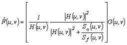
Note that the power spectrum of the noise and the original image are included in the Weiner filter which are shown below.

The power spectrum is similar to the modulus of the degradation transfer function as in the following equation.

As usual the first factor in the right hand side of the expression above denotes the complex conjugate of H(u, v).
In most cases, the power spectrum of the noise and undergraded image are not known, hence the Weiner filter can be approximated in the expression as follows.

Instead of the power spectra, it is replaced by K which is a constant that can be varied.

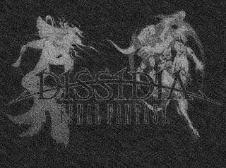
At first, the following grayscale image is obtained from the internet.

Source: http://tvtropes.org/pmwiki/pmwiki.php/Main/Ptitlefjcz80qe

A Gaussian noise with mean and standard deviation of 0.02 is then applied to the image. Next, the degradation transfer function parameters a, b, and T are varied resulting to the set of images as shown below (Arranged from top to bottom, left to right).

For T = 1: (1) a = 0.1, b = 0.1; (2) a = 0.01, b = 0.01; (3) a = 0.001, b = 0.001

For a = 0.01, b = 0.01: (1) T = 0.01; (2) T = 0.1; (3) T = 10; (4) T = 100

For constant exposure time, it can be observed that the degraded image becomes more discernible as the blurring displacements a and b decrease. Meanwhile, for constant blurring displacements, the added Gaussian noise is masked by the blurred image as the exposure time T increases.
Shown as follows are the restored images using Weiner filtering with the spectrum of the noise and undergraded image for different degradation transfer function parameters (Arranged from top to bottom, left to right).

For T = 1: (1) a = 0.1, b = 0.1; (2) a = 0.01, b = 0.01; (3) a = 0.001, b = 0.001

For a = 0.01, b = 0.01: (1) T = 0.01; (2) T = 0.1; (3) T = 10; (4) T = 100

Apparently, the restoration approaches the original image as the blurring displacements decrease as well as the exposure time increases.
The following last set of images is composed of restored images using Weiner filter with varying K values (Arranged from top to bottom, left to right).

For a = 0.01, b = 0.01, T = 1: (1) K = 0; (2) K = 0.000001; (3) K = 0.00001; (4) K = 0.0001; (5) K = 0.001; (6) K = 0.01; (7) K = 0.1; (8) K = 1

It can be noticed that since a constant, which is based from the ratio of the power spectrum of the noise to the undergraded image, is added in all the elements of the matrix in the process Weiner filtering, the added Gaussian noise is eliminated at the same time magnifying the blurring effect as K increases.
Weiner filtering with the power spectrum of the noise and the undergraded image is then recommended to be used when the power spectrum of the added noise and the undergraded image is known and also with minimal degradation while Weiner filtering with the constant K is more applicable for various corrupted image even without the power spectra as long as K is carefully chosen.

Since I am able to demonstrate a corrupted image with motion blur and additive noise, and restore it using Weiner filtering successfully, I grade myself 10/10.

I have worked individually in this activity however I have shared my insights to my classmates.

Appendix
The Scilab code below is utilized in this activity.

stacksize(4e7);

image = gray_imread('dissidia.jpg');
//scf(0);
//imshow(image, []);
//imwrite(normal(image), 'bwdissidia.bmp');

s = size(image);

noise_gauss = grand(s(1), s(2), 'nor', 0.02, 0.02);
noisy_image = image + noise_gauss;

N = fft2(noise_gauss);
F = fft2(image);

a = 0.01;
b = 0.01;
T = 1;

H = [];
for i = 1:s(1)
for j = 1:s(2)
H(i, j) = (T/(%pi*(i*a + j*b)))*(sin(%pi*(i*a + j*b)))*exp(-%i*%pi*(i*a + j*b));
end
end

G = H.*F + N;
noisy_blurred = abs(ifft(G));

//scf(1);
//imshow(noisy_blurred, []);
//imwrite(normal(noisy_blurred), 'noisy blurred_a001_b001_T1.bmp');

SN = N.*conj(N);
SF = F.*conj(F);
restore1 = (((1)./H).*((H.*conj(H))./((H.*conj(H)) + (SN./SF)))).*G;
restore1 = abs(ifft(restore1));

//scf(2);
//imshow(restore1, []);
//imwrite(normal(restore1), 'restore_a001_b001_T1.bmp');

K = 0.01;
restore2 = (((1)./H).*((H.*conj(H))./((H.*conj(H)) + K))).*G;
restore2 = abs(ifft(restore2));

//scf(3);
//imshow(restore2, []);
//imwrite(normal(restore2), 'restoreK001.bmp');

Activity 18 - Noise Models and Basic Image Restoration

In this activity, various noise models are applied in grayscale images, then different basic image restoration techniques are tested in recovering the original images.

Like in a grayscale image, noise is characterized by a probability distribution function (PDF). However, its PDF consists of random variables with parameters such as mean and standard deviation that may be altered.
The following are the most common noise models encountered in image processing. First below is the PDF of Gaussian noise which obviously follows a Gaussian curve with mu as its mean and sigma as its standard deviation.

The random variable z represents the grayscale value in the noise.
The PDF of Rayleigh noise is given as follows.

Its mean and variance are the following.

Next below is the PDF of Erlang or Gamma noise.

Whereas its mean and variance are shown as follows.

PDF of exponential noise is described by the following equations.

Its mean and variance are shown below.

Uniform noise has the following PDF.

Then its mean and variance are as follows.

Lastly, impulse or better known as salt-and-pepper noise is considered here. This has PDF expressed below.

Meanwhile, there are four basic image restoration techniques implemented in this activity. These are spatial filters which reduce added noise in the image.
Arithmetic mean filter operates through the following equation.

S_xy is a set of coordinates within a chosen rectangular sub-image window with size m x n in the noisy image centered at (x, y). Hence, it filters the noise by averaging the grayscale value at (x, y).
A noisy image under geometric mean filtering works with the equation as follows.

The harmonic mean filter which is shown below works well for salt noise or noisy pixels with grayscale values close to white but not with pepper noise or noisy pixels with grayscale values near to black.

Lastly, contraharmonic mean filter has expression given by the following.

The variable Q is called the order of the filter which may be positive that is good for pepper noise or negative that eliminates salt noise. Hence, it cannot remove both noise simultaneously.

Initially, a grayscale image as follows is created from Paint which only consists of three grayscale values.

Its PDF with grayscale values ranging from 0 to 255 is plotted in the following figure.

Apparently, the three peaks correspond to the three grayscale values of the image. Then, using the built-in function grand of Scilab, majority of the noise models are generated with the same size as the image (150 x 150). The image degradation is then simulated by simply adding the generated noise to the test image. Note that the parameters such as mean and standard deviation of the noise models in grand are carefully set to prevent the merging of the three grayscale levels in the original or test image and so the noisy image is still recognizable.
After adding Gaussian noise with mean 0.5 and standard deviation of 0.075 to the image, the image and its PDF becomes the following.

As can be observed, the Gaussian profiles have maximum near the three grayscale values implying that the noisy image is still discernable. The next set of figures are the filtered images using the arithmetic, geometric, harmonic, and contraharmonic mean filter arranged from left to right, top to bottom.

The sub-image window used for all the filters has size 3 x 3. However, the algorithm does not apply at the corners and edges of the noisy image, thus necessary boundary conditions are considered at these locations. For the contraharmonic mean filter, Q is equal to 1. It can be observed that the arithmetic and the contraharmonic mean filters are better compared in the geometric and harmonic mean filter for the added Gaussian noise.
Next, the Rayleigh noise is generated by first downloading a module called modnum. Rayleigh noise generator can then be used when the loader file of the module is loaded. The function genrayl in the module is then used with noise generator parameter set to 0.1. The resulting noisy image and its PDF after adding the Rayleigh noise are shown below.

The filtered images are as follows.

In this type of noise, all filters work well in restoring the test image.
Gamma noise is then added to the test image again using grand. Its parameters shape and scale are set to 1 and 10 respectively. The following are the resulting noisy image and its PDF.

The figures with Gamma noise after using the four filters are shown below.

The contraharmonic mean filter somehow fails in restoring the test image for the Gamma noise while the harmonic mean filter is the best filter for this case.
The test image with added exponential noise and its PDF are as follows. The mean of the exponential noise is set to 0.1.

Notice that the PDF is similar when Gamma noise is applied. The following set of figures is the result after using the four filters in the test image with Gamma noise.

And so the filtered images are similar to the added Gamma noise.
Again from grand, another noise model which is uniform noise is generated here where a uniform distribution is set from 0 to 0.2. Shown below are the noisy image and its PDF with this uniform noise.

The PDF indeed illustrate a uniform random grayscale values within the range of the three graylevels. Then, the restored noisy images with uniform noise through the four filters are as follows.

Noting that uniform noise is present, the four filters are effective in enhancing the noisy image.
The impulse or salt-and-pepper noise is simulated through the function imnoise where the noise density or probability of making salt or pepper noise is set to 0.01. The resulting noisy image and its PDF are the following.

The PDF is similar to the PDF of the test image without any noise because impulse noise only adds white (salt) or black (pepper) pixels while the test image is composed of only white, black, and gray pixels. Thus, what is only different in this PDF is the frequency of the three graylevels. Illustrated below are the filtered noisy image with impulse noise through the four filters.

It can be observed that the arithmetic mean filter is best in the test image with impulse noise. It is proven here that the harmonic mean filter eliminates salt noise but fails in pepper noise. Meanwhile, the contraharmonic mean filter with Q = 1 removes pepper noise but some salt noise still remain. Different Q values of the contraharmonic mean filter are also tested here. The filtered noisy image with Q equals to -1, 2, -2, and 0 arranged from left to right, top to bottom are as follows.

From the results above, positive Q values in the contraharmonic mean filter indeed eliminate pepper noise and not salt noise while negative Q values are truly good to salt noise but not to pepper noise. However, with Q equal to 0, both salt and pepper noise are minimized.

The whole process is also tested for a grayscale image which is not restricted to only three discrete grayscale values. The grayscale image of a beach obtained from the internet is shown below.

Source: http://www.advimglib.com/samples.html

The PDF of the image above is shown as follows.

Apparently, the PDF of this test image does not contain only three graylevels. The test image with Gaussian noise and its PDF are the following.

Below are the filtered test image with Gaussian noise using the four filters.

The test image with Rayleigh noise and its PDF are as follows.

The results of the filtered test image with Rayleigh noise through the four filters are the following.

Shown below are the test image with Gamma noise and its PDF.

The filtered test image with Gamma noise using the four filters are as follows.

Next are the test image with exponential noise and its PDF.

The following set of figures is the filtered test image with exponential noise.

Then, the test image with uniform noise and its PDF are shown below.

The filtered test image with uniform noise after applying the four filters are as follows.

Lastly, the following are the test image with impulse noise and its PDF.

Below are the filtered test image with impulse noise through the four filters.

The Q values of the contraharmonic mean filter are also varied to -1, 2, -2, and 0 resulting to the figures as follows.

Since the test image now has distribution of grayscale values, the four filters resulted to almost the same filtered image except in the test image with impulse noise unlike in the test image with only three grayscale values where a certain filter is preferred over the others. Overall, it can be deduced that the arithmetic mean filter is consistent in restoring both test image with three discrete graylevels and with distributed grayscale values to every type of noise added.

I grade myself 10/10 because I am able to simulate all the noise models introduced in this activity and I have successfully implemented the four basic image restoration techniques in the test images with different the noise models applied to them.

I thank Neil in providing me the test image with only three grayscale values.

Appendix
Below is the whole Scilab code utilized in this activity.

stacksize(4e7);

image = gray_imread('beach.jpg');
s = size(image);

//scf(0);
//imshow(image, []);

a = 1;
grayscale = [];
pixels = [];
for i = 0:255
[x, y] = find(round(255*normal(image)) == i);
grayscale(a) = i;
pixels(a) = length(x);
a = a + 1;
end

//scf(1);
//plot(grayscale, normal(pixels));
//title('PDF of Image without Noise');
//xlabel('Grayscale Values');

noise_gauss = grand(s(1), s(2), 'nor', 0.5, 0.075);
noise_ray = matrix(genrayl(0.1, s(1)*s(2)), s(1), s(2));
noise_gamma = grand(s(1), s(2), 'gam', 1, 10);
noise_exp = grand(s(1), s(2), 'exp', 0.1);
noise_uni = grand(s(1), s(2), 'unf', 0, 0.2);
noisy_image_salt = imnoise(image, 'salt & pepper', 0.01);

//noisy_image = round(255*normal(noisy_image_salt));
noisy_image = round(255*normal(image + noise_gauss));

//scf(2);
//imshow(noisy_image, []);
//imwrite(normal(noisy_image), 'image gauss noise.bmp');

a = 1;
grayscale = [];
pixels = [];
for i = 0:255
[x, y] = find(round(255*normal(noisy_image)) == i);
grayscale(a) = i;
pixels(a) = length(x);
a = a + 1;
end

//scf(3);
//plot(grayscale, normal(pixels));
//title('PDF of Image with Gaussian Noise');
//xlabel('Grayscale Values');

// Filtering Noisy Image

// Arithmetic Mean Filter

// Size of Rectangle Subimage Window (3 x 3)
m = 3;
n = 3;

for a = 1:s(1)
for b = 1:s(2)
if a == 1 & b == 1
g1 = [noisy_image(a, b) noisy_image(a, b + 1); noisy_image(a + 1, b) noisy_image(a + 1, b + 1)];
filtered1(a, b) = (1/(2*2))*sum(g1);
elseif a == 1 & b == s(2)
g1 = [noisy_image(a, b - 1) noisy_image(a, b); noisy_image(a + 1, b - 1) noisy_image(a + 1, b)];
filtered1(a, b) = (1/(2*2))*sum(g1);
elseif a == s(1) & b == 1
g1 = [noisy_image(a - 1, b) noisy_image(a - 1, b + 1); noisy_image(a, b) noisy_image(a, b + 1)];
filtered1(a, b) = (1/(2*2))*sum(g1);
elseif a == s(1) & b == s(2)
g1 = [noisy_image(a - 1, b - 1) noisy_image(a - 1, b); noisy_image(a, b - 1) noisy_image(a, b)];
filtered1(a, b) = (1/(2*2))*sum(g1);
elseif a == 1 & b ~= 1 & b ~= s(2)
g1 = [noisy_image(a, b - 1) noisy_image(a, b) noisy_image(a, b + 1); noisy_image(a + 1, b - 1) noisy_image(a + 1, b) noisy_image(a + 1, b + 1)];
filtered1(a, b) = (1/(2*3))*sum(g1);
elseif b == 1 & a ~= 1 & a ~= s(1)
g1 = [noisy_image(a - 1, b) noisy_image(a - 1, b + 1); noisy_image(a, b) noisy_image(a, b + 1); noisy_image(a + 1, b) noisy_image(a + 1, b + 1)];
filtered1(a, b) = (1/(3*2))*sum(g1);
elseif b == s(2) & a ~= 1 & a ~= s(1)
g1 = [noisy_image(a - 1, b - 1) noisy_image(a - 1, b); noisy_image(a, b - 1) noisy_image(a, b); noisy_image(a + 1, b - 1) noisy_image(a + 1, b)];
filtered1(a, b) = (1/(3*2))*sum(g1);
elseif a == s(1) & b ~= 1 & b ~= s(2)
g1 = [noisy_image(a - 1, b - 1) noisy_image(a - 1, b) noisy_image(a - 1, b + 1); noisy_image(a, b - 1) noisy_image(a, b) noisy_image(a, b + 1)];
filtered1(a, b) = (1/(2*3))*sum(g1);
else
g1 = [noisy_image(a - 1, b - 1) noisy_image(a - 1, b) noisy_image(a - 1, b + 1); noisy_image(a, b - 1) noisy_image(a, b) noisy_image(a, b + 1); noisy_image(a + 1, b - 1) noisy_image(a + 1, b) noisy_image(a + 1, b + 1)];
filtered1(a, b) = (1/(m*n))*sum(g1);
end
end
end

//scf(4);
//imshow(filtered1, []);
//imwrite(normal(filtered1), 'gauss filtered1.bmp');

// Geometric Mean Filter

for a = 1:s(1)
for b = 1:s(2)
if a == 1 & b == 1
g2 = [noisy_image(a, b) noisy_image(a, b + 1); noisy_image(a + 1, b) noisy_image(a + 1, b + 1)];
filtered2(a, b) = prod(g2)^(1/(2*2));
elseif a == 1 & b == s(2)
g2 = [noisy_image(a, b - 1) noisy_image(a, b); noisy_image(a + 1, b - 1) noisy_image(a + 1, b)];
filtered2(a, b) = prod(g2)^(1/(2*2));
elseif a == s(1) & b == 1
g2 = [noisy_image(a - 1, b) noisy_image(a - 1, b + 1); noisy_image(a, b) noisy_image(a, b + 1)];
filtered2(a, b) = prod(g2)^(1/(2*2));
elseif a == s(1) & b == s(2)
g2 = [noisy_image(a - 1, b - 1) noisy_image(a - 1, b); noisy_image(a, b - 1) noisy_image(a, b)];
filtered2(a, b) = prod(g2)^(1/(2*2));
elseif a == 1 & b ~= 1 & b ~= s(2)
g2 = [noisy_image(a, b - 1) noisy_image(a, b) noisy_image(a, b + 1); noisy_image(a + 1, b - 1) noisy_image(a + 1, b) noisy_image(a + 1, b + 1)];
filtered2(a, b) = prod(g2)^(1/(2*3));
elseif b == 1 & a ~= 1 & a ~= s(1)
g2 = [noisy_image(a - 1, b) noisy_image(a - 1, b + 1); noisy_image(a, b) noisy_image(a, b + 1); noisy_image(a + 1, b) noisy_image(a + 1, b + 1)];
filtered2(a, b) = prod(g2)^(1/(3*2));
elseif b == s(2) & a ~= 1 & a ~= s(1)
g2 = [noisy_image(a - 1, b - 1) noisy_image(a - 1, b); noisy_image(a, b - 1) noisy_image(a, b); noisy_image(a + 1, b - 1) noisy_image(a + 1, b)];
filtered2(a, b) = prod(g2)^(1/(3*2));
elseif a == s(1) & b ~= 1 & b ~= s(2)
g2 = [noisy_image(a - 1, b - 1) noisy_image(a - 1, b) noisy_image(a - 1, b + 1); noisy_image(a, b - 1) noisy_image(a, b) noisy_image(a, b + 1)];
filtered2(a, b) = prod(g2)^(1/(2*3));
else
g2 = [noisy_image(a - 1, b - 1) noisy_image(a - 1, b) noisy_image(a - 1, b + 1); noisy_image(a, b - 1) noisy_image(a, b) noisy_image(a, b + 1); noisy_image(a + 1, b - 1) noisy_image(a + 1, b) noisy_image(a + 1, b + 1)];
filtered2(a, b) = prod(g2)^(1/(m*n));
end
end
end

//scf(5);
//imshow(filtered2, []);
//imwrite(normal(filtered2), gauss filtered2.bmp');

// Harmonic Mean Filter

small_number = 0.000001;
for a = 1:s(1)
for b = 1:s(2)
if a == 1 & b == 1
g3 = [noisy_image(a, b) noisy_image(a, b + 1); noisy_image(a + 1, b) noisy_image(a + 1, b + 1)];
filtered3(a, b) = (2*2)/(sum((1)./(g3 + small_number)));
elseif a == 1 & b == s(2)
g3 = [noisy_image(a, b - 1) noisy_image(a, b); noisy_image(a + 1, b - 1) noisy_image(a + 1, b)];
filtered3(a, b) = (2*2)/(sum((1)./(g3 + small_number)));
elseif a == s(1) & b == 1
g3 = [noisy_image(a - 1, b) noisy_image(a - 1, b + 1); noisy_image(a, b) noisy_image(a, b + 1)];
filtered3(a, b) = (2*2)/(sum((1)./(g3 + small_number)));
elseif a == s(1) & b == s(2)
g3 = [noisy_image(a - 1, b - 1) noisy_image(a - 1, b); noisy_image(a, b - 1) noisy_image(a, b)];
filtered3(a, b) = (2*2)/(sum((1)./(g3 + small_number)));
elseif a == 1 & b ~= 1 & b ~= s(2)
g3 = [noisy_image(a, b - 1) noisy_image(a, b) noisy_image(a, b + 1); noisy_image(a + 1, b - 1) noisy_image(a + 1, b) noisy_image(a + 1, b + 1)];
filtered3(a, b) = (2*3)/(sum((1)./(g3 + small_number)));
elseif b == 1 & a ~= 1 & a ~= s(1)
g3 = [noisy_image(a - 1, b) noisy_image(a - 1, b + 1); noisy_image(a, b) noisy_image(a, b + 1); noisy_image(a + 1, b) noisy_image(a + 1, b + 1)];
filtered3(a, b) = (3*2)/(sum((1)./(g3 + small_number)));
elseif b == s(2) & a ~= 1 & a ~= s(1)
g3 = [noisy_image(a - 1, b - 1) noisy_image(a - 1, b); noisy_image(a, b - 1) noisy_image(a, b); noisy_image(a + 1, b - 1) noisy_image(a + 1, b)];
filtered3(a, b) = (3*2)/(sum((1)./(g3 + small_number)));
elseif a == s(1) & b ~= 1 & b ~= s(2)
g3 = [noisy_image(a - 1, b - 1) noisy_image(a - 1, b) noisy_image(a - 1, b + 1); noisy_image(a, b - 1) noisy_image(a, b) noisy_image(a, b + 1)];
filtered3(a, b) = (2*3)/(sum((1)./(g3 + small_number)));
else
g3 = [noisy_image(a - 1, b - 1) noisy_image(a - 1, b) noisy_image(a - 1, b + 1); noisy_image(a, b - 1) noisy_image(a, b) noisy_image(a, b + 1); noisy_image(a + 1, b - 1) noisy_image(a + 1, b) noisy_image(a + 1, b + 1)];
filtered3(a, b) = (m*n)/(sum((1)./(g3 + small_number)));
end
end
end

//scf(6);
//imshow(filtered3, []);
//imwrite(normal(filtered3), 'gauss filtered3.bmp');

// Contraharmonic Mean Filter

Q = 0;
for a = 1:s(1)
for b = 1:s(2)
if a == 1 & b == 1
g4 = [noisy_image(a, b) noisy_image(a, b + 1); noisy_image(a + 1, b) noisy_image(a + 1, b + 1)];
filtered4(a, b) = (sum((g4 + small_number).^(Q + 1)))/(sum((g4 + small_number).^Q));
elseif a == 1 & b == s(2)
g4 = [noisy_image(a, b - 1) noisy_image(a, b); noisy_image(a + 1, b - 1) noisy_image(a + 1, b)];
filtered4(a, b) = (sum((g4 + small_number).^(Q + 1)))/(sum((g4 + small_number).^Q));
elseif a == s(1) & b == 1
g4 = [noisy_image(a - 1, b) noisy_image(a - 1, b + 1); noisy_image(a, b) noisy_image(a, b + 1)];
filtered4(a, b) = (sum((g4 + small_number).^(Q + 1)))/(sum((g4 + small_number).^Q));
elseif a == s(1) & b == s(2)
g4 = [noisy_image(a - 1, b - 1) noisy_image(a - 1, b); noisy_image(a, b - 1) noisy_image(a, b)];
filtered4(a, b) = (sum((g4 + small_number).^(Q + 1)))/(sum((g4 + small_number).^Q));
elseif a == 1 & b ~= 1 & b ~= s(2)
g4 = [noisy_image(a, b - 1) noisy_image(a, b) noisy_image(a, b + 1); noisy_image(a + 1, b - 1) noisy_image(a + 1, b) noisy_image(a + 1, b + 1)];
filtered4(a, b) = (sum((g4 + small_number).^(Q + 1)))/(sum((g4 + small_number).^Q));
elseif b == 1 & a ~= 1 & a ~= s(1)
g4 = [noisy_image(a - 1, b) noisy_image(a - 1, b + 1); noisy_image(a, b) noisy_image(a, b + 1); noisy_image(a + 1, b) noisy_image(a + 1, b + 1)];
filtered4(a, b) = (sum((g4 + small_number).^(Q + 1)))/(sum((g4 + small_number).^Q));
elseif b == s(2) & a ~= 1 & a ~= s(1)
g4 = [noisy_image(a - 1, b - 1) noisy_image(a - 1, b); noisy_image(a, b - 1) noisy_image(a, b); noisy_image(a + 1, b - 1) noisy_image(a + 1, b)];
filtered4(a, b) = (sum((g4 + small_number).^(Q + 1)))/(sum((g4 + small_number).^Q));
elseif a == s(1) & b ~= 1 & b ~= s(2)
g4 = [noisy_image(a - 1, b - 1) noisy_image(a - 1, b) noisy_image(a - 1, b + 1); noisy_image(a, b - 1) noisy_image(a, b) noisy_image(a, b + 1)];
filtered4(a, b) = (sum((g4 + small_number).^(Q + 1)))/(sum((g4 + small_number).^Q));
else
g4 = [noisy_image(a - 1, b - 1) noisy_image(a - 1, b) noisy_image(a - 1, b + 1); noisy_image(a, b - 1) noisy_image(a, b) noisy_image(a, b + 1); noisy_image(a + 1, b - 1) noisy_image(a + 1, b) noisy_image(a + 1, b + 1)];
filtered4(a, b) = (sum((g4 + small_number).^(Q + 1)))/(sum((g4 + small_number).^Q));
end
end
end

//scf(7);
//imshow(filtered4, []);
//imwrite(normal(filtered4), 'gauss filtered4.bmp');