The barrel geometric distortion in an image is removed in this activity based on the image's pixel coordinates and graylevel values.
The following distorted image of a grid is obtained from the internet.

Source: http://www.jmg-galleries.com/blog/2007/08/01/photo-term-series-post-13-barrel-distortion
The correction starts with the image's pixel coordinates. A subgrid from a distorted image can be thought of transformation of this subgrid from the ideal image through functions in the horizontal and vertical coordinates as shown below.


The transformation of a vertex from a subgrid is then illustrated as follows.

The following transformation functions are thus bilinear if the vertex from the ideal image is mapped simultaneously in both directions.


Eight equations are enough to determine the unknown eight coefficients c_1 to c_8 and these come from the two coordinates of the four vertices of a closed region in the grid both in the distorted and ideal image. Hence, a different set of coefficients is yielded for other closed region.
Initially from the distorted image obtained from the internet, a vertex from the most undistorted region is located. In this case, it is approximately near the image's center. Then, the length in pixels of the ideal rectangle is measured. The size of the ideal rectangle in the grid is found to be 28 x 28 pixels. Starting from the vertex, the pixel coordinates by counting 28 pixels to its left, right, top and bottom are determined and so the vertex points of the ideal grid are generated which is shown as follows.

Notice that the pixel coordinates at the edges are also obtained in order to cover the whole distorted image in correcting the barrel distortion. Meanwhile, the pixel coordinates of the vertices in the distorted image corresponding to the ideal image are gathered using the function locate of Scilab.
The sets of coefficients for each rectangle are then determined from the following equations.

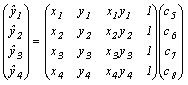
The matrix expressions can be rewritten as follows.


So the coefficients are computed as shown below.


Now, per pixel inside a rectangle, the coordinates from the distorted image are attained using the corresponding set of coefficients in that rectangle through the following equations.


The grayscale values of each pixel are the next to be handled. At first, a matrix of zeros with the same size of the distorted image (150 x 151) is created. Then, interpolated graylevel values of each computed locations in the distorted image are copied to this blank matrix.
Two types of graylevel interpolation are implemented here. The first one is the nearest neighbor interpolation technique where the graylevel value of the nearest integer-valued coordinate is used and this just comes from the rounded pixel coordinates in the distorted image calculated using the eight coefficients.
Bilinear graylevel interpolation is the second technique employed to correct the barrel distortion. Since many of the computed pixel coordinates in the distorted image are not integer-valued, this technique is expected to result to a better corrected image compared to the nearest neighbor graylevel interpolation. Otherwise, the graylevel value at integer-valued locations is automatically copied to the blank matrix. An illustration of bilinear graylevel interpolation is shown below.

The pixel location pointed above is clearly not integer-valued. Through the equation below, the graylevel value is obtained at this location.

Notice that the equation above has form exactly the same in calculating the pixel coordinates in the distorted image. Thus, the same procedure applies in the bilinear graylevel interpolation which is based from the matrix expression shown as follows.

The coefficients a, b, c, and d must first be determined using four equations. These are then coming from the four nearest pixels of each computed pixel coordinate in the distorted image. The integer coordinates are assumed to be at the center of each pixel hence the four nearest pixels are located at the rounded values of 0.5 pixel away from calculated pixel location in the distorted image for both directions. The 4 x 4 matrix from the expression above are then assembled for each computed pixel coordinate in the distorted image which contains the location of the four nearest pixels. The following is the simplified version of the matrix expression above.

Then, the coefficients a, b, c, and d for each computed pixel location in the distorted image are acquired as shown below.

The interpolated graylevel value of each calculated pixel location in the distorted image is then transferred to the blank matrix for each pixel inside a rectangle in the ideal grid. The whole algorithm is repeated for the other rectangles in the ideal grid.
Recall that vertices at the perimeter of the ideal grid and distorted image are also considered. Thus to prevent incorrect indexing, the graylevel value is directly copied from the distorted image onto the black matrix at the pixel coordinate inside a rectangle in the ideal grid, if the calculated pixel location is less than 1 or greater than the length of the image which is 150 for the vertical direction and 151 for the horizontal direction.
The next figure is the result of the nearest neighbor graylevel interpolation technique applied to the barrel distorted grid image.

It can be observed that the lines are pixelated and jagged even though the curved grid lines are straightened.
Meanwhile, the figure below is the result of the bilinear graylevel interpolation.

Apparently, bilinear graylevel interpolation is better than the nearest neighbor interpolation technique. The barrel distortion is completely eliminated at the same time producing smooth grid lines.
I say that this activity has the most complicated code so far but since I have successfully corrected the barrel distortion of a grid image and understand how the whole process is implemented, I grade myself 10/10.
Earl has helped me in this activity and I thank Mandy for explaining how she has implemented the bilinear graylevel interpolation technique.
Appendix
The following Scilab code is utilized in this activity.
The following distorted image of a grid is obtained from the internet.

Source: http://www.jmg-galleries.com/blog/2007/08/01/photo-term-series-post-13-barrel-distortion
The correction starts with the image's pixel coordinates. A subgrid from a distorted image can be thought of transformation of this subgrid from the ideal image through functions in the horizontal and vertical coordinates as shown below.


The transformation of a vertex from a subgrid is then illustrated as follows.
The following transformation functions are thus bilinear if the vertex from the ideal image is mapped simultaneously in both directions.


Eight equations are enough to determine the unknown eight coefficients c_1 to c_8 and these come from the two coordinates of the four vertices of a closed region in the grid both in the distorted and ideal image. Hence, a different set of coefficients is yielded for other closed region.
Initially from the distorted image obtained from the internet, a vertex from the most undistorted region is located. In this case, it is approximately near the image's center. Then, the length in pixels of the ideal rectangle is measured. The size of the ideal rectangle in the grid is found to be 28 x 28 pixels. Starting from the vertex, the pixel coordinates by counting 28 pixels to its left, right, top and bottom are determined and so the vertex points of the ideal grid are generated which is shown as follows.

Notice that the pixel coordinates at the edges are also obtained in order to cover the whole distorted image in correcting the barrel distortion. Meanwhile, the pixel coordinates of the vertices in the distorted image corresponding to the ideal image are gathered using the function locate of Scilab.
The sets of coefficients for each rectangle are then determined from the following equations.


The matrix expressions can be rewritten as follows.


So the coefficients are computed as shown below.


Now, per pixel inside a rectangle, the coordinates from the distorted image are attained using the corresponding set of coefficients in that rectangle through the following equations.


The grayscale values of each pixel are the next to be handled. At first, a matrix of zeros with the same size of the distorted image (150 x 151) is created. Then, interpolated graylevel values of each computed locations in the distorted image are copied to this blank matrix.
Two types of graylevel interpolation are implemented here. The first one is the nearest neighbor interpolation technique where the graylevel value of the nearest integer-valued coordinate is used and this just comes from the rounded pixel coordinates in the distorted image calculated using the eight coefficients.
Bilinear graylevel interpolation is the second technique employed to correct the barrel distortion. Since many of the computed pixel coordinates in the distorted image are not integer-valued, this technique is expected to result to a better corrected image compared to the nearest neighbor graylevel interpolation. Otherwise, the graylevel value at integer-valued locations is automatically copied to the blank matrix. An illustration of bilinear graylevel interpolation is shown below.

The pixel location pointed above is clearly not integer-valued. Through the equation below, the graylevel value is obtained at this location.

Notice that the equation above has form exactly the same in calculating the pixel coordinates in the distorted image. Thus, the same procedure applies in the bilinear graylevel interpolation which is based from the matrix expression shown as follows.

The coefficients a, b, c, and d must first be determined using four equations. These are then coming from the four nearest pixels of each computed pixel coordinate in the distorted image. The integer coordinates are assumed to be at the center of each pixel hence the four nearest pixels are located at the rounded values of 0.5 pixel away from calculated pixel location in the distorted image for both directions. The 4 x 4 matrix from the expression above are then assembled for each computed pixel coordinate in the distorted image which contains the location of the four nearest pixels. The following is the simplified version of the matrix expression above.

Then, the coefficients a, b, c, and d for each computed pixel location in the distorted image are acquired as shown below.

The interpolated graylevel value of each calculated pixel location in the distorted image is then transferred to the blank matrix for each pixel inside a rectangle in the ideal grid. The whole algorithm is repeated for the other rectangles in the ideal grid.
Recall that vertices at the perimeter of the ideal grid and distorted image are also considered. Thus to prevent incorrect indexing, the graylevel value is directly copied from the distorted image onto the black matrix at the pixel coordinate inside a rectangle in the ideal grid, if the calculated pixel location is less than 1 or greater than the length of the image which is 150 for the vertical direction and 151 for the horizontal direction.
The next figure is the result of the nearest neighbor graylevel interpolation technique applied to the barrel distorted grid image.

It can be observed that the lines are pixelated and jagged even though the curved grid lines are straightened.
Meanwhile, the figure below is the result of the bilinear graylevel interpolation.

Apparently, bilinear graylevel interpolation is better than the nearest neighbor interpolation technique. The barrel distortion is completely eliminated at the same time producing smooth grid lines.
I say that this activity has the most complicated code so far but since I have successfully corrected the barrel distortion of a grid image and understand how the whole process is implemented, I grade myself 10/10.
Earl has helped me in this activity and I thank Mandy for explaining how she has implemented the bilinear graylevel interpolation technique.
Appendix
The following Scilab code is utilized in this activity.
stacksize(4e7);
distort = gray_imread('barrel_distortion.jpg');
pixelx = 28;
pixely = 28;
tran = 20;
s = size(distort);
ideal = zeros(s(1), s(2));
xit = [];
yit = [];
for i = 1:5
for j = 1:5
xit = [xit, tran + pixelx*(j - 1)];
yit = [yit, tran + pixely*(i - 1)];
ideal(tran + pixelx*(i - 1), tran + pixely*(j - 1)) = 1;
end
end
xit = matrix(xit, 5, 5);
yit = matrix(yit, 5, 5);
xi = zeros(7, 7);
yi = zeros(7, 7);
xi(2:6, 2:6) = xit;
yi(2:6, 2:6) = yit;
xi(1,:) = 1;
xi(7,:) = s(1);
yi(:,1) = 1;
yi(:,7) = s(2);
ideal(1, 1) = 1;
ideal(1, s(2)) = 1;
ideal(s(1), 1) = 1;
ideal(s(1), s(2)) = 1;
for k = 1:5
xi(k + 1, 1) = xi(k + 1, 2);
xi(k + 1, 7) = xi(k + 1, 2);
yi(1, k + 1) = yi(2, k + 1);
yi(7, k + 1) = yi(2, k + 1);
ideal(xi(k + 1, 2), 1) = 1;
ideal(1, yi(2, k + 1)) = 1;
ideal(xi(k + 1, 2), s(2)) = 1;
ideal(s(1), yi(2, k + 1)) = 1;
end
//scf(0);
//imshow(ideal);
//imwrite(ideal, 'idealgrid.bmp');
//scf(1);
//imshow(distort, []);
//xdyd = (locate(49, 1))';
//fprintfMat('xdyd.txt', xdyd);
xdyd = fscanfMat('xdyd.txt');
xd = s(1) - xdyd(:,2);
yd = xdyd(:,1);
xd = (matrix(xd', 7, 7))';
yd = (matrix(yd', 7, 7))';
newgrid_bilinear = zeros(s(1), s(2));
newgrid_nearest_neighbor = zeros(s(1), s(2));
for a = 1:6
for b = 1:6
vertex_upperleft = [xd(a, b), yd(a, b)];
vertex_upperright = [xd(a, b + 1), yd(a, b + 1)];
vertex_lowerleft = [xd(a + 1, b), yd(a + 1, b)];
vertex_lowerright = [xd(a + 1, b + 1), yd(a + 1, b + 1)];
xd4 = [vertex_upperleft(1); vertex_upperright(1); vertex_lowerleft(1); vertex_lowerright(1)];
yd4 = [vertex_upperleft(2); vertex_upperright(2); vertex_lowerleft(2); vertex_lowerright(2)];
T = [xi(a, b) yi(a, b) xi(a, b)*yi(a, b) 1; xi(a, b + 1) yi(a, b + 1) xi(a, b + 1)*yi(a, b + 1) 1; xi(a + 1, b) yi(a + 1, b) xi(a + 1, b)*yi(a + 1, b) 1; xi(a + 1, b + 1) yi(a + 1, b + 1) xi(a + 1, b + 1)*yi(a + 1, b + 1) 1];
C1to4 = inv(T)*xd4;
C5to8 = inv(T)*yd4;
for m = (xi(a, 1)):(xi((a + 1), 1))
for n = (yi(1, b)):(yi(1, (b + 1)))
points_in_one_box = [m n m*n 1];
xnew = points_in_one_box*C1to4;
ynew = points_in_one_box*C5to8;
rxnew = round(xnew);
rynew = round(ynew);
if xnew < 1 | xnew > s(1) | ynew < 1 | ynew > s(2)
newgrid_bilinear(m, n) = distort(m, n);
newgrid_nearest_neighbor(m, n) = distort(m, n);
else
if xnew - rxnew == 0 & ynew - rynew == 0
newgrid_bilinear(m, n) = distort(xnew, ynew);
else
nearest_lowerleft = [round(xnew - 0.5), round(ynew - 0.5)];
nearest_upperleft = [round(xnew - 0.5), round(ynew + 0.5)];
nearest_lowerright = [round(xnew + 0.5), round(ynew - 0.5)];
nearest_upperright = [round(xnew + 0.5), round(ynew + 0.5)];
nearest_pixels = [nearest_lowerleft(1) nearest_lowerleft(2) nearest_lowerleft(1)*nearest_lowerleft(2) 1; nearest_upperleft(1) nearest_upperleft(2) nearest_upperleft(1)*nearest_upperleft(2) 1; nearest_lowerright(1) nearest_lowerright(2) nearest_lowerright(1)*nearest_lowerright(2) 1; nearest_upperright(1) nearest_upperright(2) nearest_upperright(1)*nearest_upperright(2) 1];
distortgray_lowerleft = distort(nearest_lowerleft(1), nearest_lowerleft(2));
distortgray_upperleft = distort(nearest_upperleft(1), nearest_upperleft(2));
distortgray_lowerright = distort(nearest_lowerright(1), nearest_lowerright(2));
distortgray_upperright = distort(nearest_upperright(1), nearest_upperright(2));
distortgray_nearest = [distortgray_lowerleft; distortgray_upperleft; distortgray_lowerright; distortgray_upperright];
abcd_coefficients = inv(nearest_pixels)*distortgray_nearest;
interpolated_gray = [xnew ynew xnew*ynew 1]*abcd_coefficients;
newgrid_bilinear(m, n) = interpolated_gray;
newgrid_nearest_neighbor(m, n) = distort(rxnew, rynew);
end
end
end
end
end
end
//scf(2);
//imshow(newgrid_bilinear, []);
//imwrite(newgrid_bilinear/max(newgrid_bilinear), 'newgrid_bilinear.bmp');
//scf(3);
//imshow(newgrid_nearest_neighbor, []);
//imwrite(newgrid_nearest_neighbor/max(newgrid_nearest_neighbor), 'newgrid_nearest_neighbor.bmp');
No comments:
Post a Comment